A Theory of Saddle Escape in Deep Nonlinear Networks
Analyzing training dynamics in small-initialization deep nonlinear neural networks [arXiv]
(Part of a series of short writeups covering recent work.)
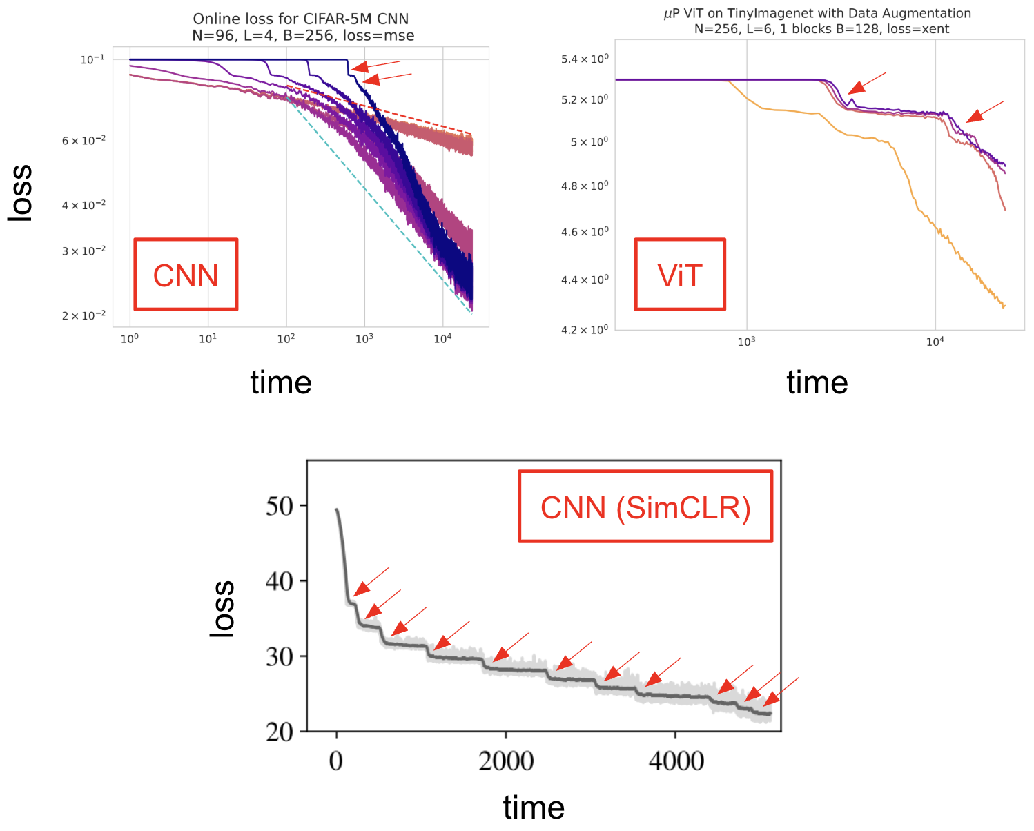
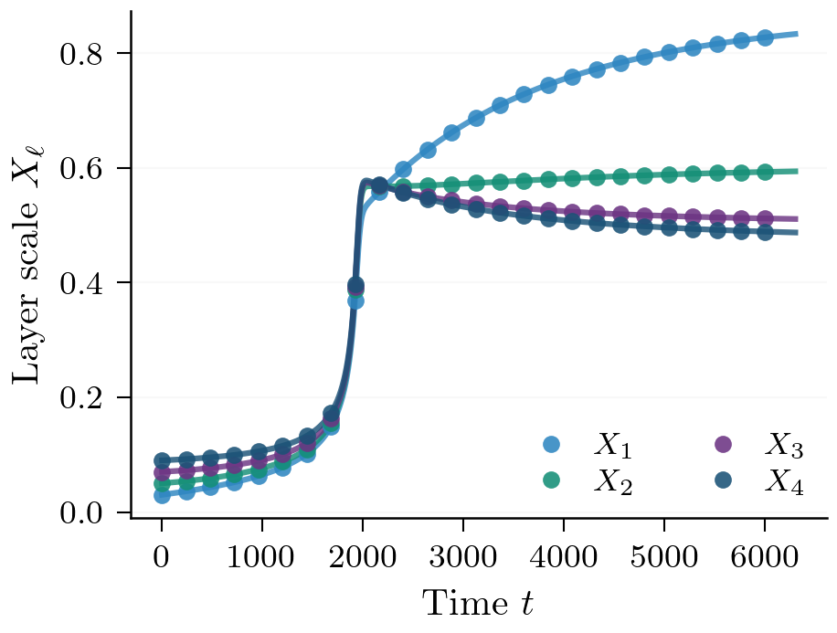
Training deep networks from small initialization has a characteristic pattern: long plateaus where the loss barely moves, then sharp drops as new features are learned. This "saddle-to-saddle" structure is well understood for linear networks, where an exact conservation law makes the training flow tractable. For nonlinear activations, the conservation law that underlies much of the deep linear network literature breaks, and it isn't clear what should replace it, or what controls how long each plateau lasts. In this work, we identify the right replacement: an exact identity governing the imbalance between adjacent layer norms, valid for any smooth activation and any differentiable loss. The identity is used to determine that escape time depends not on the total depth, but only on the number of bottleneck layers.1
- We derive an exact identity for the imbalance that holds for any smooth activation and differentiable loss, and use it to classify activations into four universality classes.
- We show that on the permutation-symmetric manifold, the full matrix flow reduces to a scalar ODE, giving escape time controlled by the number of bottleneck layers , not total depth .
- We show the same exponent is recovered under He-normal initialization via a signal energy bootstrap argument.
Background
Linear Networks
A lot of the existing theory for training dynamics in deep networks is built on the deep linear network model: an -layer network with no activation function, just a chain of matrix multiplications . Despite their simplicity, deep linear networks exhibit nontrivial dynamics under gradient flow, and many features of deep learning (e.g. saddle-to-saddle structure, low-rank bias, progressive feature learning) appear here in analytically tractable form [SMG14].
The main object is the imbalance of the weight matrix norms between adjacent layers: For linear networks, the imbalance is exactly conserved along gradient flow: for all and all . This is because the linear activation satisfies Euler's homogeneity identity exactly: for .2 So the functional vanishes identically. This conservation reduces the full high-dimensional matrix flow to a much simpler scalar system, and it is the foundation of most deep linear network analyses.
The Problem with Nonlinear Activations
For a general nonlinear activation , : the imbalance is no longer conserved and starts to drift. A natural question to ask here is by how much, and what exactly controls the rate?
The answer depends on the Taylor expansion of near zero.3 Writing , the leading nonzero term has some order . For tanh: , so , giving . For a quadratic activation , one gets , so .
Near the saddle, pre-activations (the value passed into the activation) are small (order ), so is tiny -- the drift is slow and the dynamics look almost linear. The order governs exactly how slow, and therefore governs the escape time. To make this precise, we will need the imbalance identity.
Imbalance Identity
Having identified as the right object to track, we can now state our main technical tool. Consider an -layer network with pre-activations and population loss .
Theorem 1 (Imbalance Identity). For any smooth activation and any differentiable loss ,
Two things to notice. First, the identity is exact. Second, the right-hand side is a correlation between the upstream gradient at layer and applied to the pre-activations at layer . When (the linear case), the right-hand side vanishes and we recover exact conservation. When , the drift rate is controlled by how large is -- and near the saddle, where , this is .
Activation Classes
The order of the first nonlinear term in classifies activations into four universality classes:
- Class A (): Linear activations and ReLU. The imbalance is exactly conserved; the nonlinear network behaves like a linear one at leading order.4
- Class B (first term odd, order ): tanh, GELU, and other odd-symmetric activations. For tanh, , so .
- Class C (first term even, order ): activations with a nonzero quadratic term in . The drift is faster than Class B for the same .
- Class D (constant offset, ): sigmoid and other activations with nonzero mean. The constant term in dominates near the origin, and the dynamics are qualitatively different.
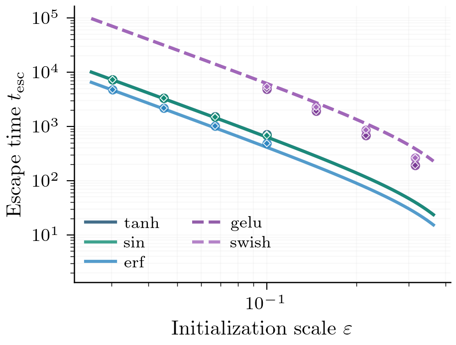
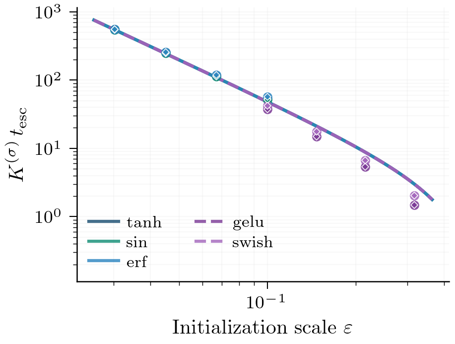
Two activations in the same class with the same exhibit the same escape time up to a computable prefactor ; after rescaling by , their escape curves collapse.5 Here, escape time means the time the loss escapes the first saddle, i.e. the time the first plateau ends.
Symmetric Manifold Ansatz
The imbalance identity tells us exactly how the matrix flow drifts. But to actually solve for the escape time, we need to reduce the full -dimensional matrix gradient flow to something tractable. The way we do this is to restrict to the permutation-symmetric submanifold: the set of configurations where every weight matrix has identical rows.6
On this submanifold, the forward pass collapses completely. Each layer just multiplies a scalar by the shared row magnitude, then applies pointwise. So the entire network output is a composition of scalar multiplications and univariate activations -- an -dimensional system in the row magnitudes rather than a system in the full weight entries.
This reduction is exact and has two key properties:
- Flow-invariant: if you initialize on the symmetric submanifold, gradient flow keeps you there for all time. The gradient at any point on the submanifold points back into the submanifold.
- Imbalance identity closes: on the submanifold, the identity becomes a scalar equation in . Combined with an approximate balance law7 that keeps the close to each other near the saddle, the full -dimensional system reduces to a single scalar ODE.
The scalar ODE is what makes the escape time calculable exactly.
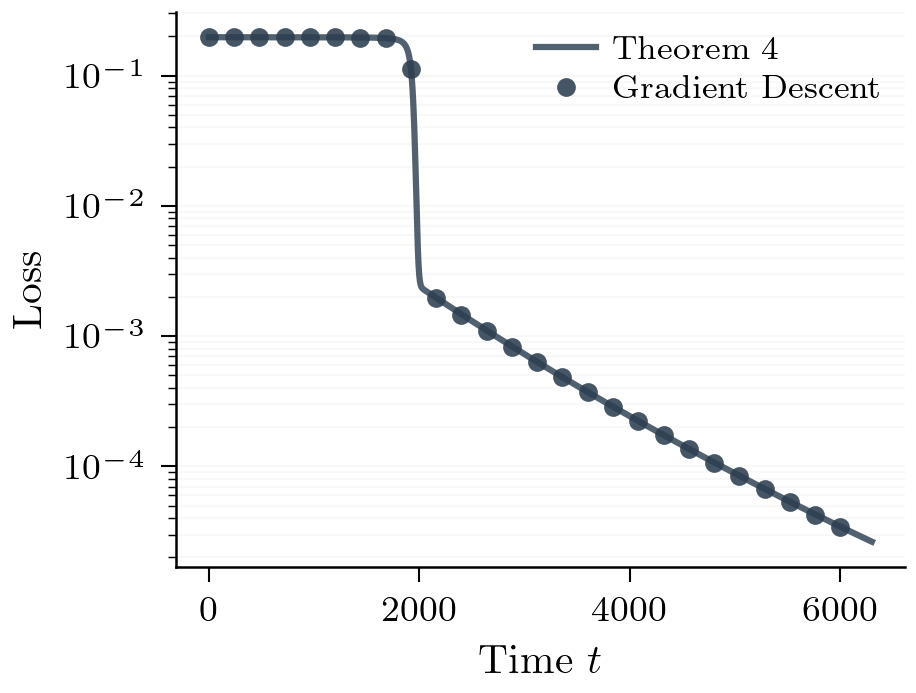
Critical-Depth Law
With the scalar reduction in hand, we can now compute the escape time exactly. Suppose of the layers initialize at scale (call this the bottleneck) and the remaining layers initialize at scale . By symmetry, all bottleneck layers have the same scalar magnitude .
The gradient driving each bottleneck layer is the product of the signals through all the other bottleneck layers, so it scales as . The full-size layers contribute factors and only affect the prefactor. The scalar ODE for the shared bottleneck magnitude is therefore Starting from and integrating until : This integral has three regimes depending on :
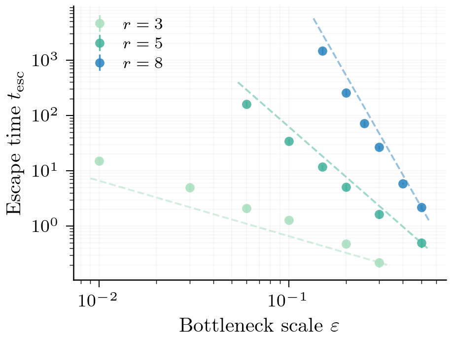
Theorem 2 (Critical-Depth Escape Law). As , the escape time satisfies
The exponent has a pretty neat interpretation: one power of is consumed because each layer's gradient is rather than (the layer itself doesn't appear in its own gradient), and a second is absorbed by the integral. Total depth drops out entirely -- the layers set the prefactor but not the exponent. The threshold at is special: it is the minimal bottleneck for which the escape time diverges as .8
Off-Manifold
The scalar reduction is satisfying, but it raises an obvious concern: real networks don't initialize on the symmetric manifold. Does the same escape time law hold under a generic initialization like He-normal?
The answer is yes, but the argument works differently. Rather than reducing to a scalar system via the ansatz, we use a single scalar quantity that can be defined for any weight configuration: the signal energy9 where and are specific functions of the network's input-output map.10 Near the saddle, is small (order ). As training progresses, grows, and escape corresponds to reaching an threshold.
The key is that satisfies a differential inequality of the form which can be integrated directly: starting from , the time to reach is . The same exponent as on the manifold, with no ansatz required.
The proof works in two stages. First, a bootstrap interval is identified where the operator norms of the weight matrices remain controlled, so the signal energy inequality holds. Second, a filtered composition argument shows that the gradient mass at each layer is dominated by the product structure , which is what drives the growth. Together, these give the same exponent that emerges from the symmetric manifold. The symmetric manifold is preserved by the flow but is not attracting (generic initializations drift away from it) yet the escape time exponent is robust to this drift.
A No-Go Theorem
The single-mode theory is great and all, but a natural next step is to extend it to multi-mode teachers: networks that must learn several features in sequence, escaping a chain of saddles one at a time. The tool to try is the row-moment hierarchy; a system of equations tracking the moments of the row distributions of each , generalizing the scalar to multi-mode settings.
This doesn't work, and not for a fixable reason.11
Theorem 3 (No-Closure of the Row-Moment Hierarchy). The row-moment hierarchy does not admit finite closure. No finite set of moments satisfies a closed ODE system under the gradient flow for a multi-mode teacher.
This is a hard impossibility: you can't get a finite-dimensional reduction by tracking any fixed set of moments. Any complete theory of successive saddle-escape times requires fundamentally different machinery.
The second obstruction is geometric. In the single-mode case, the symmetric manifold is flow-invariant, which is what makes the scalar reduction valid. For multi-mode teachers, the analogous structure is the block-aligned ansatz. Unlike the single-mode case, this ansatz is not flow-invariant: linearizing the gradient flow around stage- saddles reveals positive eigenvalues in the off-block directions whenever the mixed loop gain exceeds one.12 Generic initializations drift away from the block structure, and the reduction breaks.
- A nonlinear analog of the "get rich quick" phenomenon of [KRD+24]. ↩
- This is quite easy to verify yourself, and will be the basis of the rest of the paper. ↩
- This is just the first instance of using the physicist's toolkit; a number of the ideas and techniques in the paper are inspired by physics. ↩
- ReLU is linear almost everywhere, so we just group it in with linear. ↩
- Specifically, , where is the leading Taylor coefficient of , is the leading coefficient of , and is the linear coefficient of . ↩
- Formally, each for a shared direction and scalar ; the "identical rows" condition means all rows of are the same vector. ↩
- Near the saddle, all bottleneck layers initialize at the same scale , and the imbalance identity implies the imbalances drift slowly -- at rate for Class B. So the stay approximately equal throughout the escape, justifying the scalar reduction. ↩
- At the special depth (e.g. for tanh where ), two scales in the normal form align and the leading-order terms don't dominate cleanly, producing an extra correction on top of the power law. We don't discuss it much in the paper since there's already a lot going on, but perhaps an interesting avenue for future work! (or maybe not since it's a measure zero event) ↩
- Yet another physics-y style thing. ↩
- Concretely, captures the network's input-output correlation and is a related quantity from the loss gradient. The product measures how much useful signal is flowing through the network end-to-end. ↩
- This is a no-go theorem, similar to those given to prove the existence of quantum mechanics, e.g. Bell's Theorem or "Not in our Stars" (from one of Andrew Charman's QM exams). ↩
- This is actually inspired largely by a discussion we had in one of my classes, which is summed up really nicely in [Rec20]. ↩
References
- [KRD+24]Daniel Kunin et al. Get rich quick: exact solutions reveal how unbalanced initializations promote rapid feature learning. 2024. [link] ↩
- [Rec20]Ben Recht. There are none. 2020. [link] ↩
- [SMG14]Andrew M. Saxe, James L. McClelland, and Surya Ganguli. Exact solutions to the nonlinear dynamics of learning in deep linear neural networks. 2014. [link] ↩