Rao-Blackwellized Score Matching on Manifolds

A lot of modern machine learning assumes the manifold hypothesis: the assumption that the data we care about has some structure to it (formally, this means that it lies on or near some manifold). Under the manifold hypothesis, score matching (a widely used method for learning a data distribution) is fundamentally ill-posed. As a result, practitioners use a variant known as denoising score matching, which resolves the ill-posedness problem, but doesn't necessarily guarantee that we learn the right data distribution. In this work, we examine what exactly is learned by denoising score matching.

Background

Score Matching

A lot of times, we want to learn a data distribution, but we can't because computing the partition function¹ is intractable. So, instead of matching the distribution's values at every point in the domain, we instead match the gradient [Hyv05] (this gets rid of our partition function problem because the partition function is independent of the coordinate $x$). This works fantastically for general data, but if we constrain our data to lie on some low dimensional structure, things fall apart rather quickly. Since the probability distribution is nonzero on the manifold, but zero right off the manifold, we have points at which the derivative does not exist and score matching is not well defined. To get around this, we add noise to the data so that it no longer lies exactly on the manifold.²

Denoising score matching. The practical way to do this is denoising score matching (DSM): we take a clean sample $Z \sim q$ (here $q$ is our data distribution defined on the manifold), corrupt it with Gaussian noise to get $X \doteq Z + \sigma\xi$ for $\xi \sim \mathcal{N}(0, I_D)$, and train a network to regress against the denoising direction $(Z-X)/\sigma^2$. By Tweedie's formula [Efr11], minimizing this regression loss recovers the score of the noisy density $q_\sigma = q * \phi_\sigma$, and as $\sigma \to 0^+$, this converges to the score of $q$ itself. When $q$ is a nice density on $\mathbb R^D$, we are done: DSM gives you the score up to a $\sigma^2$ smoothing bias.

But under the manifold hypothesis the ambient score doesn't exist at all ($q$ has no density w.r.t. the Lebesgue measure), so there is nothing to take the gradient of. DSM at $\sigma > 0$ is still a well-defined regression problem, it's just not clear what exactly it's estimating. To start thinking about this, it's helpful to split the denoising direction at each noisy point $X$ into pieces along and orthogonal to the manifold (denoted $M$ from here on out) at the nearest projection $\pi(X) \in M$. The normal piece is just $(\pi(X) - X)/\sigma^2$, a deterministic function of $X$ -- so it contains no information about where $Z$ actually came from on $M$. All the signal lives in the tangent piece: $$T_\sigma \doteq \frac{1}{\sigma^2} P_{T_{\pi(X)} M}(Z - X) \in T_{\pi(X)} M.$$

This leaves a few questions open: what is $T_\sigma$ actually estimating? Does it converge to the intrinsic Riemannian score $\nabla_M \log q$? Does it even have a sensible variance as $\sigma \to 0^+$?

In order to answer these, we'll need to set up a bit of differential geometry.

Differential Geometry

Differential geometry is concerned with differentiable manifolds: geometric structures that, when we zoom in enough, look like regular flat (Euclidean) space.³ For example, a plane embedded in a three-dimensional space is a manifold. A plane is a special type of manifold since it doesn't have any curvature: most manifolds have two notions of curvature.

Curvature. Extrinsic curvature tells us how $M$ bends inside the ambient $\mathbb{R}^D$. Intrinsic curvature is inherent to $M$ and requires no knowledge of the embedding in ambient space. Both end up as linear maps on the tangent space, so we may compare them directly.

At each $z \in M$, the ambient space splits as $\mathbb{R}^D = T_z M \oplus N_z M$, with orthogonal projections $P_{T_z M}$ and $P_{N_z M}$.

Second fundamental form, Weingarten operator, and mean curvature. Consider traveling along $M$ in some tangent direction $u$. The velocity vector can't stay constant in $\mathbb{R}^D$; the manifold is curving, so $u$ must bend. The part of that bending that points normal to $M$ is the second fundamental form: $II_z(u, v) \in N_z M$, a symmetric bilinear map on $T_z M \times T_z M$. It's a super clean object for measuring extrinsic curvature since it directly measures how tangent directions get pushed off the manifold. The Weingarten operator is the exact same information, just in the form of a linear map. For each normal direction $\nu \in N_z M$, define $W_\nu : T_z M \to T_z M$ by $\langle W_\nu u, v \rangle = \langle II_z(u, v), \nu \rangle$. $W_\nu$ acts on tangent vectors, so we can apply it directly to things like $\nabla_M \log q(z)$ -- which is what shows up in the result. The mean curvature vector is the trace of $II$: $H(z) \doteq \sum_i II_z(e_i, e_i) \in N_z M$ for any orthonormal basis $(e_i)$ of $T_z M$ (the sum is basis-independent). This points in the direction $M$ is curving "on average."

Gauss equation. Intrinsic and extrinsic curvature are actually linked: the metric on $M$ is induced from the ambient inner product. The exact relationship is given by the Gauss equation $\mathrm{Ric}_z^\sharp = W_{H(z)} - \sum_\alpha W_{n_\alpha}^2$, where $(n_\alpha)$ is any orthonormal basis of $N_z M$. The takeaway is that intrinsic curvature is determined by the embedding: it's the mean-curvature Weingarten minus a separate "sum of squared Weingartens" contribution.

Rao-Blackwellization and the Nearest-Point Projection

Having established our machinery, we may now return to the question we really care about: what is $T_\sigma$ actually estimating, and can we control its variance?

The classical statistics move here is Rao-Blackwellization. The Rao-Blackwell Theorem tells us that conditioning an unbiased estimator on a sufficient statistic can only reduce its variance. Intuitively, we keep the expected value, but integrate out the part of the noise that doesn't carry any signal. The natural thing to condition on in our setting is the nearest-point projection $\pi(X) \in M$. It captures the manifold-valued summary of the noisy observation -- "where on $M$ did $Z$ likely come from" -- and discards the normal offset, which by construction carries no information about $Z$. Formally, among all fiber-collapsing summaries $S(X)$ -- statistics depending on $X$ only through $\pi(X)$, i.e. $\sigma(S) \subseteq \sigma(\pi(X))$ -- the projection $\pi(X)$ is the finest. Anything coarser throws away information that $\pi(X)$ retains.

Define the Rao-Blackwellized tangent target: $r_\sigma(z) \doteq \mathbb{E}\bigl[T_\sigma \mid \pi(X) = z\bigr] \in T_z M$. From the Pythagorean identity for $L^2$ projections, we can show that among all functions $h$ of $\pi(X)$, the choice $h(\pi(X)) = r_\sigma(\pi(X))$ minimizes the regression risk: $$\mathbb{E}|T_\sigma - h(\pi(X))|^2 = \mathbb{E}|T_\sigma - r_\sigma(\pi(X))|^2 + \mathbb{E}|r_\sigma(\pi(X)) - h(\pi(X))|^2.$$

Thus, $r_\sigma$ is the unique (up to null sets) $L^2$-optimal target in this class, and the excess risk of any coarser estimator decomposes into the irreducible "noise" part and a separable "estimator error" part. Intuitively, $r_\sigma$ keeps all the signal-bearing information in $T_\sigma$ and averages out the rest.

Variance Collapse

The conditional variance of $T_\sigma$ given $\pi(X)$ is the irreducible portion that can't be removed by any fiber-collapsing summary, and we can write it down exactly:

The intuition for the $d/\sigma^2$ is pretty straightforward. Conditioned on $\pi(X) = z$, the latent $Z$ is concentrated on $M$ within a tangent ball of radius $\sim \sigma$ around $z$ (this is just the posterior of $Z$ given $X$). So $Z - X$ has typical tangent magnitude $\sim \sigma$, and dividing by $\sigma^2$ gives a typical magnitude of $1/\sigma$. Squaring and summing over the $d$ tangent dimensions gives $d/\sigma^2$. So, as we shrink the noise, the variance of $T_\sigma$ grows, which is exactly the opposite of what we want from a regression target.

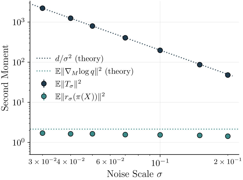
The $d/\sigma^2$ floor isn't just a property of our particular estimator -- it's an irreducible Bayes-risk floor for any fiber-collapsing summary. That is, for any statistic $S(X)$ with $\sigma(S) \subseteq \sigma(\pi(X))$, the best possible $L^2$ predictor of $T_\sigma$ based on $S$ has expected squared error at least $d/\sigma^2 + O(1)$. Coarsening $\pi(X)$ doesn't help; only the projection itself achieves the floor exactly.

$\sigma^2$ Correction

Now that we have a target with bounded variance, the natural next question is what it actually equals. Expanding $r_\sigma(z)$ as a power series in $\sigma$: $$r_\sigma(z) = \nabla_M \log q(z) + \sigma^2 \bigl[b_q(z) + g_M^{\text{ext}}(z)\bigr] + o(\sigma^2),$$ uniformly on $M$.

The leading term is the intrinsic Riemannian score $\nabla_M \log q$ -- exactly what fully-intrinsic methods regress against. So at leading order, ambient DSM (after the Rao-Blackwellization fix) recovers the right thing. The $\sigma^2$ correction is more interesting. It splits into two distinct pieces:

1. The intrinsic Tweedie bias $b_q(z) = \frac{1}{2} \nabla_M\left(\Delta_M \log q + |\nabla_M \log q|^2\right)$. This is the manifold analog of the flat-Tweedie bias: it comes from Gaussian smoothing of the density and would appear even on a flat support. It depends on $q$ but not on the embedding, and it's the same correction you'd get from intrinsic methods.
2. The extrinsic curvature term $g_M^{\text{ext}}(z) = \bigl(\tfrac{1}{2} W_{H(z)} - \mathrm{Ric}_z^\sharp\bigr)\nabla_M \log q(z)$. This piece matters for non-flat manifolds. It depends on the embedding of $M$ in $\mathbb{R}^D$ via the Weingarten and Ricci operators defined before. It's invisible to any method that corrupts $Z$ by intrinsic Riemannian noise -- intrinsic noise never leaves the manifold, and thus never feels the embedding.

A nice property of $g_M^{\text{ext}}$ is that the operator $\tfrac{1}{2} W_H - \mathrm{Ric}^\sharp$ is purely geometric -- it depends only on how $M$ sits in $\mathbb{R}^D$, not on $q$. So if we've trained a score model $\hat s(z) \approx \nabla_M \log q(z)$, we can apply this operator to our model's output and subtract $\sigma^2$ times the result. The correction is fully post-hoc; you don't need to re-train, and you don't need to know $q$.⁶

$S^2$ Cancellation

On $S^d \subset \mathbb{R}^{d+1}$, $W_\nu = -\mathrm{Id}$, $H(z) = -dz$, $W_{H(z)} = d \mathrm{Id}$, and $\mathrm{Ric}^\sharp = (d-1) \mathrm{Id}$. Plugging in: $$g_{S^d}^{\text{ext}}(z) = \bigl(\tfrac{d}{2} - (d-1)\bigr) \mathrm{Id} \cdot \nabla_{S^d}\log q(z) = (1 - d/2) \nabla_{S^d}\log q(z).$$ So on the sphere, the extrinsic correction is a scalar multiple of the intrinsic score, with coefficient $\alpha_d \doteq 1 - d/2$:

• $d = 1$: $\alpha_1 = +1/2$;
• $d = 2$: $\alpha_2 = 0$;
• $d = 3$: $\alpha_3 = -1/2$;
• $d \geq 4$: increasingly negative.

On $S^2$, the extrinsic curvature correction vanishes identically, and ambient DSM recovers the intrinsic score up to only the flat-Tweedie bias $b_q$.

It's worth emphasizing that this is a coincidence specific to the round sphere, not a general 2-manifold property. The torus $T^2 \subset \mathbb{R}^3$ is intrinsically flat ($\mathrm{Ric}^\sharp = 0$) but extrinsically curved, and the corresponding $g_{T^2}^{\text{ext}}$ has coefficient $+1/2$ -- a measurable embedding-only bias. Higher-dimensional spheres also show the bias clearly: on $S^6$ and $S^{10}$, raw ambient DSM under-concentrates the equilibrium distribution by about 17% and 33% respectively, both removed by the post-hoc correction.

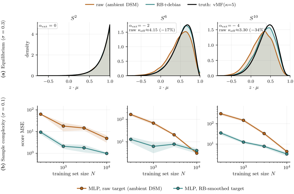
This explains a longstanding empirical observation: ambient diffusion models work surprisingly well on most test cases such as climate or weather data, which naturally live on $S^2$.

References

- [Efr11]Bradley Efron. "Tweedie’s Formula and Selection Bias". Journal of the American Statistical Association Vol. 106, pp. 1602 - 1614 2011. [link] ↩
- [Hyv05]Aapo Hyvärinen. "Estimation of non-normalized statistical models by score matching". 2005. [link] ↩
- [doC92]Manfredo Perdigão do Carmo. Riemannian Geometry. 1992. ↩